1. 线性模型
有监督学习是通过已知的样本产生预测模型的学习方法,任何有监督学习模型都可被想象成一个函数:
\[y=f(x_1,x_2,x_3,…x_n) \tag{1-1}\]
其中,\(x_1,x_2,x_3…x_n\)是模型的n维的特征值,\(y\)是要预测的目标值/分类,当\(y\)是可枚举的类型时,对应分类问题(classification);\(y\)为连续值时,该模型解决回归问题(regression)。
线性回归(Linear Regression)在机器学习中被用来解决学习特征和目标值都是连续值类型的问题,可定义为多项式函数:
\[y=w_0+w_1x_1+w_2x_2+…+w_nx_n \tag{1-2}\]
线性模型学习的目标就是确定\(w_0 w_1..w_n\)的值,使\(y\)可以根据特征值直接通过函数计算得到,\(w_0\)成为截距,\(w_1…w_n\)被成为回归系数(coefficient)。
公式(2)可以有其他变体,注意:是否是线性模型取决于其被要求的系数\(w_0…w_n\)之间是否为线性关系,与样本特征变量\(x_0..x_n\)的形式无关。e.g.以下前者为线性模型,后者为非线性模型。
\[y=2w_0+w_1x^1+w_1x^2+…w_nx^n\]\[y=w_0+sin(w_1)x_1+cos(x_2)x_2+…\]2. 最小二乘法
最简单的线性模型算法便是最小二乘法(Ordinary Least Squares, OLS),通过样本真值与预测值之间的方差和来达到计算出\(w_1,w_2..w_n\)的目的,即:
\[argmin(\sum(\hat{y}-y)^2) \tag{1-3}\]
arg min就是使后面这个式子达到最小值时的变量的取值,其中\(\hat{y}\)是样本预测值,\(y\)是样本中的真值(ground truth)
在python使用
import numpy as npfrom sklearn import linear_modelx = np.array([[0, 1], [3, -2], [2, 3]]) # 训练样本特征y = np.array([0.5, 0.3, 0.9]) # 训练样本目标值reg = linear_model.LinearRegression() # 最小二乘法回归对象reg.fit(x, y) # 训练、拟合print("intercept_:", reg.intercept_) # 读取截距# intercept_: 0.36666666666666686print("coef_:", reg.coef_) # 读取回归参数# coef_: [0.06666667 0.13333333]reg.predict([[1, 2], [-3, 9]]) # 预测# array([0.7 , 1.36666667])通过intercept_和coef_属性可知道上述代码拟合的线性模型为:
\[y=0.36666666666666686+0.06666667x_1+0.13333333x_2\]最小二乘的不足
随着特征维度的增加,模型的求得的参数\(w_0 w_2…w_n\)的值显著增加,OLS始终试图最小化公式的值,因此为了拟合训练数据中很小的\(x\)的值差异产生的较大\(y\)值差异,必须使用较大的\(w\)值,结果是任何一个微小的变化都会导致最终预测目标值大幅度变化,即过拟合。请看:
# 测试数据def make_data(nDim): x0 = np.linspace(1, np.pi, 50) # 一个维度的特征 x = np.vstack([[x0,], [i**x0 for i in range(2, nDim+1)]]) # nDim个维度的特征 y = np.sin(x0) + np.random.normal(0, 0.15, len(x0)) # 目标值 return x.transpose(), yx, y = make_data(12)使用最小二乘法拟合:
def linear_regression(): dims = [1,3,6,12] # 需要训练的维度 for idx, i in enumerate(dims): plt.subplot(2, int(len(dims)/2), idx+1) reg = linear_model.LinearRegression() sub_x = x[:, 0:i] # 取x中前i个维度的特征 reg.fit(sub_x, y) # 训练 plt.plot(x[:,0], reg.predict(sub_x)) # 绘制模型 plt.plot(x[:,0], y, '.') plt.title("dim %s"%i) print("dim %d :"%i) print("intercept_: %s"%(reg.intercept_)) # 查看截距参数 print("coef_: %s"%(reg.coef_)) # 查看回归参数 plt.show()linear_regression()## 输出# dim 1 :# intercept_: 1.5190767802159115# coef_: [-0.39131134]# dim 3 :# intercept_: 1.1976858427101735# coef_: [ 1.91353693 -1.39387114 0.16182502]# dim 6 :# intercept_: -221.70126917849046# coef_: [-104.46259453 520.30421899 -573.61812163 429.72658285 -181.37364277# 32.5448376 ]# dim 12 :# intercept_: -7992016.158635169# coef_: [-1.83126880e+06 5.87461130e+07 -2.99765476e+08 9.72248992e+08# -1.92913886e+09 2.18748658e+09 -8.81323910e+08 -1.12973621e+09# 2.01475457e+09 -1.40758872e+09 4.94058411e+08 -7.17485861e+07]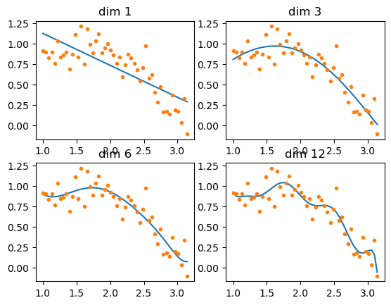
可以明显看到dim=12已经过拟合了
3. 岭回归
岭回归(Ridge Regression 或称Tikhonov Regularization)由俄罗斯科学家Tikhonov提出,通过改变回归目标系数,达到了控制回归参数随着维度疯狂增长的目的。新的回归函数:
\[argmin(\sum(\hat{y}-y)^2+\alpha\sum w^2) \tag{2-1}\]
与OLS的差别在于将\(\alpha\sum w^2\)加入最小化目标(也被称为L2惩罚项,即L2 Penalty),其中\(\alpha\)是一个可调节的超参数,\(w\)是线性模型中的所有参数。
Ridge与原来的LinearRegression类使用方法相似,只是在初始化对象需要超参数α
def ridge_regression(): alphas = [1e-15, 1e-12, 1e-5, 1, ] # α参数 for idx, i in enumerate(alphas): plt.subplot(2, int(len(alphas)/2), idx+1) reg = linear_model.Ridge(alpha=i) # 岭回归模型 sub_x = x[:, 0:12] # 取x中前i个维度的特征 reg.fit(sub_x, y) # 训练 plt.plot(x[:,0], reg.predict(sub_x)) # 绘制模型 plt.plot(x[:,0], y, '.') plt.title("dim=12, alpha=%e"%i) print("alpha %e :"%i) print("intercept_: %s"%(reg.intercept_)) # 查看截距参数 print("coef_: %s"%(reg.coef_)) # 查看回归参数 plt.show()ridge_regression()#输出结果# dim 1 :# intercept_: 1.5190767802159115# coef_: [-0.39131134]# dim 3 :# intercept_: 1.1976858427101735# coef_: [ 1.91353693 -1.39387114 0.16182502]# dim 6 :# intercept_: -221.70126917849046# coef_: [-104.46259453 520.30421899 -573.61812163 429.72658285 -181.37364277# 32.5448376 ]# dim 12 :# intercept_: -7992016.158635169# coef_: [-1.83126880e+06 5.87461130e+07 -2.99765476e+08 9.72248992e+08# -1.92913886e+09 2.18748658e+09 -8.81323910e+08 -1.12973621e+09# 2.01475457e+09 -1.40758872e+09 4.94058411e+08 -7.17485861e+07]
比较OLS模型的12维结果,模型参数\(w\)显著降低。并且\(\alpha\)参数大小与训练结果成反比:\(\alpha\)越大,回归参数越小,模型越平缓。
3. Lasso回归
Ridge已经可以解决了多特征情况下参数太大导致的过度拟合,但在该模型中,无论\(\alpha\)多大,回归模型都存在绝对值极小的参数,难以到达零值,这部分参数对最终预测结果影响甚微但消耗计算资源,因此需要将不重要的特征参数计算为零,即压缩特征。这便是Lasso回归:
\[argmin(\sum(\hat{y}-y)^2+\alpha\sum|w|) \tag{3-1}\]
对上面的代码略作修改
def lasso_regression(): alphas = [1e-12, 1e-5, 1, 10] # α参数 for idx, i in enumerate(alphas): plt.subplot(2, int(len(alphas)/2), idx+1) reg = linear_model.Lasso(alpha=i) # Lasso模型 sub_x = x[:, 0:12] # 取x中前12个维度的特征 reg.fit(sub_x, y) # 训练 plt.plot(x[:,0], reg.predict(sub_x)) # 绘制模型 plt.plot(x[:,0], y, '.') plt.title("dim=12, alpha=%e"%i) print("alpha %e :"%i) print("intercept_: %s"%(reg.intercept_)) # 查看截距参数 print("coef_: %s"%(reg.coef_)) # 查看回归参数 plt.show()lasso_regression()## 输出# alpha 1.000000e-12 :# intercept_: 0.6298258513945978# coef_: [ 1.22542814e+00 -4.54947716e-01 -3.93085543e-02 -5.49725917e-03# -5.88010501e-04 2.47220823e-04 3.36442748e-04 2.85372733e-04# 2.20237636e-04 1.66111569e-04 1.25225041e-04 9.51371122e-05]# alpha 1.000000e-05 :# intercept_: 0.6275025198172812# coef_: [ 1.21848162e+00 -4.48693464e-01 -4.01246675e-02 -5.58492834e-03# -6.02833485e-04 2.41969131e-04 3.37470151e-04 2.86500656e-04# 2.21159502e-04 1.66823390e-04 1.25767364e-04 9.55513093e-05]# alpha 1.000000e+00 :# intercept_: 0.9304502324995079# coef_: [-0.00000000e+00 -0.00000000e+00 -0.00000000e+00 -0.00000000e+00# -0.00000000e+00 -0.00000000e+00 -0.00000000e+00 -0.00000000e+00# -0.00000000e+00 -6.76060251e-04 -7.30714077e-05 -0.00000000e+00]# alpha 1.000000e+01 :# intercept_: 0.9076753246287685# coef_: [-0. -0. -0. -0. -0. -0.# -0. -0. -0. -0. -0. -0.0004185]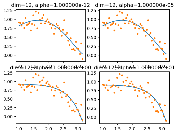
参考文献
[1]刘长龙. 从机器学习到深度学习[M]. 1. 电子工业出版社, 2019.3.